Contour Comparison

This notebook demonstrates how to compute compute contour comparison metrics using PlatiPy.

Import Modules

try:
    import platipy
except:
    !pip install platipy
    import platipy

from pathlib import Path

import pandas as pd
import SimpleITK as sitk

%matplotlib inline

from platipy.imaging.tests.data import download_and_extract_zip_file
from platipy.imaging.label.comparison import (
    compute_metric_dsc,
    compute_metric_hd,
    compute_metric_masd,
    compute_volume_metrics,
    compute_surface_metrics,
    compute_surface_dsc)
from platipy.imaging.visualisation.comparison import contour_comparison
from platipy.imaging.utils.crop import label_to_roi

Download Test Data

This will download some sample data which was generated using the TCIA LCTSC dataset. The data contains some manual contours as well as auto contours.

Note the contours in this dataset are for demonstration purposes only. No emphasis was placed on the quality of these contours.

data_path = Path("./data/contour_comparison_sample")

test_data_zip_url = "https://zenodo.org/record/7519243/files/platipy_contour_comparison_testdata.zip?download=1"

# Only download data if we haven't already downloaded the data previously
if len(list(data_path.glob("*/*.nii.gz"))) == 0:
    download_and_extract_zip_file(test_data_zip_url, data_path)

Load data

Let’s read in the data that we’ve downloaded

ct_image = sitk.ReadImage(str(data_path.joinpath("image", "CT.nii.gz")))

structure_names =["ESOPHAGUS", "HEART", "LUNG_L", "LUNG_R", "SPINALCORD"]

manual_structures = {
    s: sitk.ReadImage(str(data_path.joinpath("manual", f"{s}.nii.gz"))) for s in structure_names
}

auto_structures = {
    s: sitk.ReadImage(str(data_path.joinpath("auto", f"{s}.nii.gz"))) for s in structure_names
}

Compute Metrics (for single structure)

The following cells demonstrate computing some common metrics between the manual and auto heart contour.

heart_dsc = compute_metric_dsc(manual_structures["HEART"], auto_structures["HEART"])
print(f"Dice Similarity Coefficient for Heart is: {heart_dsc:.2f}")

Dice Similarity Coefficient for Heart is: 0.88

heart_hd = compute_metric_hd(manual_structures["HEART"], auto_structures["HEART"])
print(f"Hausdorff distance for Heart is: {heart_hd:.2f}mm")

Hausdorff distance for Heart is: 11.92mm

heart_masd = compute_metric_masd(manual_structures["HEART"], auto_structures["HEART"])
print(f"Mean Absolute Surface for Heart is: {heart_masd:.2f}mm")

Mean Absolute Surface for Heart is: 4.04mm

heart_surface_dsc = compute_surface_dsc(manual_structures["HEART"], auto_structures["HEART"])
print(f"Surface DSC for Heart with a tau of 3mm is: {heart_surface_dsc:.2f}") # 3mm is the default value for tau

heart_surface_dsc = compute_surface_dsc(manual_structures["HEART"], auto_structures["HEART"], tau=5)
print(f"Surface DSC for Heart with a tau of 5mm is: {heart_surface_dsc:.2f}")

Surface DSC for Heart with a tau of 3mm is: 0.52
Surface DSC for Heart with a tau of 5mm is: 0.72

Compute metrics (for multiple structures)

This example loops over each structure and computes some volume metrics using the compute_volume_metrics helper function. These are tracked in a list and finally converted to a pandas DataFrame.

result =  []
for structure_name in manual_structures:


    volume_dict = compute_volume_metrics(manual_structures[structure_name], auto_structures[structure_name])

    structure_dict = {
        "structure": structure_name,
        **volume_dict,
    }

    result.append(structure_dict)

df_metrics = pd.DataFrame(result)
df_metrics

	structure	DSC	volumeOverlap	fractionOverlap	truePositiveFraction	trueNegativeFraction	falsePositiveFraction	falseNegativeFraction
0	ESOPHAGUS	0.430794	9.861946	0.274530	0.357610	0.999905	0.000095	0.642390
1	HEART	0.879741	626.272202	0.785301	0.824823	0.999561	0.000439	0.175177
2	LUNG_L	0.895018	953.364372	0.809984	0.939151	0.998134	0.001866	0.060849
3	LUNG_R	0.905581	1330.435753	0.827454	0.934013	0.997875	0.002125	0.065987
4	SPINALCORD	0.647406	33.305168	0.478640	0.614366	0.999825	0.000175	0.385634

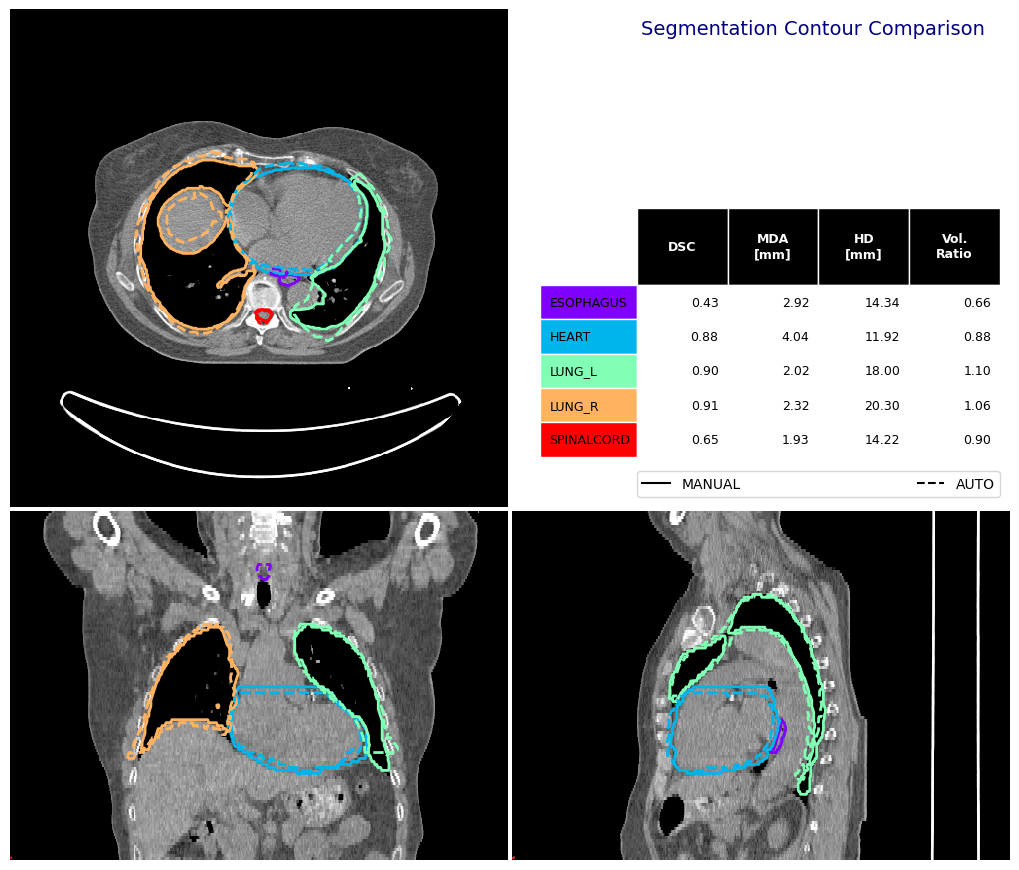
Contour Comparison Function

You can use the contour_comparison function to prepare a visualisation and return a pandas DataFrame of commonly used metrics.

fig, df_mas = contour_comparison(
    img = ct_image,
    contour_dict_a = manual_structures,
    contour_dict_b = auto_structures,
    contour_label_a = "MANUAL",
    contour_label_b = "AUTO",
    structure_for_com = "HEART",
    title='Segmentation Contour Comparison',
    subtitle='',
    subsubtitle='',
)

df_mas

	STRUCTURE	DSC	MDA_mm	HD_mm	VOL_MANUAL_cm3	VOL_AUTO_cm3
0	ESOPHAGUS	0.430794	2.916249	14.344129	27.577400	18.207550
0	HEART	0.879741	4.037049	11.917850	759.281158	664.484024
0	LUNG_L	0.895018	2.023395	18.000000	1015.133858	1115.246773
0	LUNG_R	0.905581	2.319356	20.295816	1424.428940	1513.873100
0	SPINALCORD	0.647406	1.932112	14.218965	54.210663	48.677444

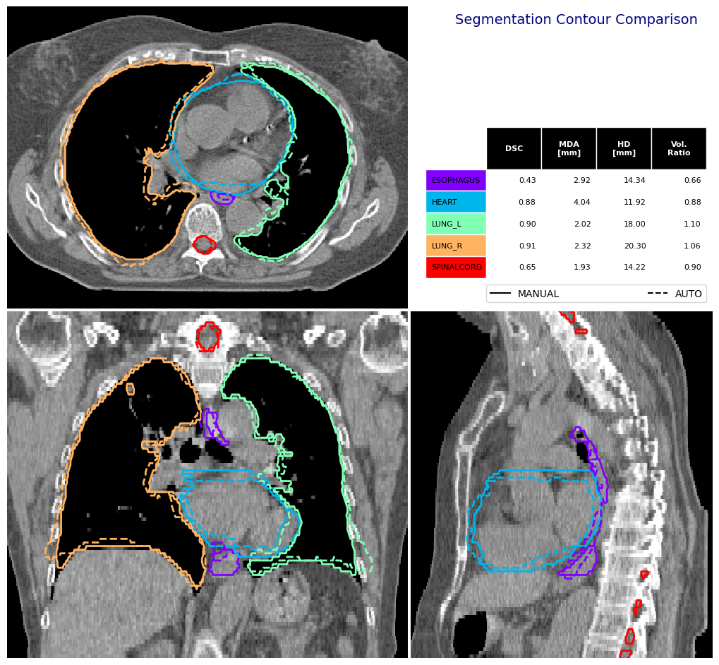
Set limits for visualisation

You can pass through a dictionary in img_vis_kw to send specific keyword arguments to the ImageVisualiser class. In this example we set the limits of the visualisation to the area of the left and right lungs combined.

(sag_size, cor_size, ax_size), (sag_0, cor_0, ax_0) = label_to_roi(
            manual_structures["LUNG_L"] | manual_structures["LUNG_R"], expansion_mm=40
        )
limits = [ax_0,
          ax_0 + ax_size,
          cor_0,
          cor_0 + cor_size,
          sag_0,
          sag_0 + sag_size,
]

fig, df_mas = contour_comparison(
    img = ct_image,
    contour_dict_a = manual_structures,
    contour_dict_b = auto_structures,
    contour_label_a = "MANUAL",
    contour_label_b = "AUTO",
    structure_for_com = "ESOPHAGUS",
    title='Segmentation Contour Comparison',
    subtitle='',
    subsubtitle='',
    img_vis_kw={"limits": limits},
)

Contour Comparison Reference

You can find a full list of all contour comparison functions in the PlatiPy documentation.